Example¶

To introduce the workings of the Simago package a basic example is supplied. With this example a population can be generated with three properties per person:

Sex: male or female
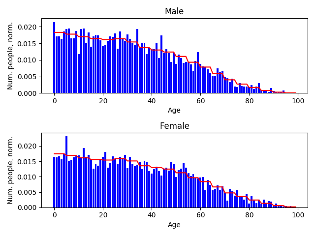
Age: 0 to 99+, dependent on the sex of the person
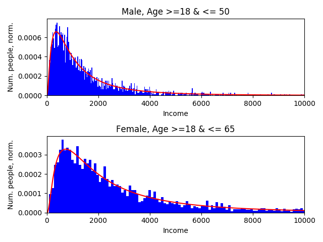
Income: A continuous lognormal distribution, dependent on the age and sex of the person.

The data for the distributions of for the properties ‘sex’ and ‘age’ are from https://www.populationpyramid.net/ for the year 2017. In the folder conversion_scripts some scripts are found to transform the downloaded CSV to the format used by Simago. The data for the income property is fictional and solely to demonstrate the functionality.

In this example the actual population is generated by calling the simago package directly and supplying some arguments via argparse. To replicate the example the following expression can be used:

python -m simago -p 1000 --yaml-folder ./data-yaml/ -o ./output/population.csv --rand_seed 100

In the Python script the following code is executed:

population = generate_population(args.popsize, args.yaml_folder, args.rand_seed)
population.update()
population.export(args.output, nowrite=args.nowrite)

In the first line the function generate_population is supplied with the population size, the path to the folder containing the settings (YAML) files and a seed for random number generation. This function then generates a PopulationClass object which contains all the information about the properties and the probability distributions as defined in the settings files. By calling population.update() the actual random values for all the defined properties and all persons in the population are drawn. After this the population is contained in the population object as the Pandas DataFrame population.population. To write this DataFrame to a file, the export() method can be called. In this case args.output is the path where to write the file. To just print the population DataFrame to the console the argument nowrite can be set to True.

Now we will walk through the way the settings and data files are defined for each of the properties.

Property: Sex¶

For each property a settings file must be defined in the form of a YAML file. For this example all the settings files for the example are stored in ./example/data-yaml/. For the property ‘sex’ this looks as follows:

property_name: "sex"
data_type: "categorical"

data_file: "../data/sex.csv"

conditions: null # null if no conditions

Every property needs to have a unique property name; in this case the obvious choice has been made. As a data type there currently are three possible options:

categorical: Discrete options with no ordering.
ordinal: Discrete options with an order in them.
continuous: Continuous values.

In the case of the sex of a person there we here consider ‘male’ and ‘female’ which makes it a categorical variable, because there is no ordering. In the data file the known data can be found, which will be used to create the probability distribution. The data file in this case looks as follows:

option,value,label,condition_index
0,3805370719,male,0
1,3742018211,female,0

The option in the first column is a unique index for each of the possible outcomes of the variable. In this case the options are 0 and 1 which each correspond to the human readable label of ‘male’ and ‘female’. In the case of the property ‘sex’ the total amount of males and females are shown. The normalized values for each option will form the discrete probability distribution.

The column for condition_index is not used for this property and in the settings file conditions is set to null. These options are used when the the probabilities for a certain property depend on another property. This will be a factor for ‘age’ and ‘income’.

Property: Age¶

The treatment of the ‘age’ is a little more complicated than the property of ‘sex’. In this case we let the age of a person depend on their sex. This follows from the data that was gathered; the age distribution is different for males and females. The settings file of the ‘age’ property is as follows:

property_name: "age"
data_type: "ordinal"

data_file: "../data/age.csv"

conditions: "../data/age_conditions.csv"

The data type in this case is ordinal because one can make an ordering of people based on their age; some people are older or younger than others. When we take a look at the data file we see (shortened for readability):

option,value,label,condition_index
0,69623692.0,0,0
1,69623692.0,1,0
2,69623692.0,2,0
...
97,202110.8,97,0
98,202110.8,98,0
99,202110.8,99,0
0,65323152.2,0,1
1,65323152.2,1,1
2,65323152.2,2,1
...
97,556794.6,97,1
98,556794.6,98,1
99,556794.6,99,1

In this case we see that some rows correspond to condition_index of 0 and others to 1. These indices match to the conditions given in the conditions file mentioned at the conditions parameter in the settings file. This conditions file looks like this:

condition_index,property_name,option,relation
0,sex,0,eq
1,sex,1,eq

Here we see two conditions corresponding to the condition index of 0 and 1. In this case the values for the options mentioned in the data file with condition_index == 0 hold when the property ‘sex’ is equal to option 0, which in this case means the sex is male. The values in the data file with condition_index == 1 correspond to option 1 for property ‘sex’ which is female. The values in the data file are normalized for each condition index. These normalized values will then form the discrete conditional probability for a person to be of a certain age given that they are of a certain sex.

Property: Income¶

Where for categorical and ordinal variables the settings files are mainly a way to indicate where the relevant files are stored, the settings files for continuous variables such as ‘income’ contain a bit more information. Let’s take a look at the settings file in this example:

property_name: "income"
data_type: "continuous"

pdf_parameters: [[1000, 1], [2000, 1]]
pdf_file: "../pdfs/pdf.py"
pdf: "pdf_lognorm"

conditions: "../data/income_conditions.csv"

For each continuous variable a continuous probability density function in the form of an ‘frozen’ rv_continuous object from the scipy.stats package needs to be supplied. An rv_continuous object becomes frozen when it is initiated with the parameters for the probability distribution specified. The name of the function for this probability density function is in this case pdf_lognorm in the file mentioned under pdf_file. Ths file looks as follows:

from scipy.stats import lognorm


def pdf_lognorm(params):
    """
    This function returns an instance of scipy.stats.norm
    with the correct paramters
    s = sigma
    scale = exp(mu)
    """
    scale = params[0]
    s = params[1]
    return lognorm(s=s, scale=scale)

The parameters for this function can be varied with the condition index. They are selected by taking the values in the position of the list pdf_parameters corresponding to the condition index. To see what these condition indices mean we look at the conditions file:

condition_index,property_name,option,relation
0,sex,0,eq
0,age,18,geq
0,age,50,leq
1,sex,1,eq
1,age,18,geq
1,age,65,leq

Multiple conditions for each condition_index are combined. In this case condition_index of 0, and therefore the parameters [1000, 1] correspond to every person that

is male,
has an age greater than or equal to 18
and less than or equal to 50.

The parameters [2000, 1] associated with a condition_index of 1 are for every person that

is female,
has an age greater than or equal to 18
and less than or equal to 65.

Probability and Population objects¶

All the information on each of the properties is each encapsulated in their own ProbabilityClass object. All the ProbabilityClass objects of the properties are then incorporated into a PopulationClass object. By calling the update() method of the PopulationClass object the values are drawn from the (conditional) probability distributions that were supplied.

Resulting data¶

If we look at the resulting data, we see that the characteristics roughly match the supplied aggregated data. This is what we expected seen as these values are all randomly drawn.

Sex	Original	Generated
Male	0.504	0.508
Female	0.496	0.492